library(rpact)
packageVersion("rpact") Defining Group Sequential Boundaries with rpact
Planning
This document provides example code for the the definition of the most commonly used group sequential boundaries in rpact.
Introduction
In rpact, sample size calculation for a group sequential trial proceeds by following the same two steps regardless of whether the endpoint is a continuous, binary, or a time-to-event endpoint:
- Define the (abstract) group sequential boundaries of the design using the function
getDesignGroupSequential(). - Calculate sample size for the endpoint of interest by feeding the abstract boundaries from step 1 into specific functions for the endpoint of interest. This step uses functions such as
getSampleSizeMeans()(for continuous endpoints),getSampleSizeRates()(for binary endpoints), andgetSampleSizeSurvival()(for survival endpoints).
The mathematical rationale for this two-step approach is that all group sequential trials, regardless of the chosen endpoint type, rely on the fact that the \(z\)-scores at different interim stages follow the same “canonical joint multivariate distribution” (at least asymptotically).
This document covers the more abstract first step, step 2 is not covered in this document but it is covered in the separate endpoint-specific R Markdown files for continuous, binary, and time-to-event endpoints. Of note, step 1 can be omitted for trials without interim analyses.
These examples are not intended to replace the official rpact documentation and help pages but rather to supplement them.
In general, rpact supports both one-sided and two-sided group sequential designs. If futility boundaries are specified, however, only one-sided tests are permitted. For simplicity, it is often preferred to use one-sided tests for group sequential designs (typically, with \(\alpha = 0.025\)).
First, load the rpact package
[1] '4.4.0'Designs with efficacy interim analyses
O’Brien & Fleming type \(\alpha\)-spending
Example:
- Interim analyses at information fractions 33%, 67%, and 100% (
informationRates = c(0.33, 0.67, 1)). [Note: For equally spaced interim analyses, one can also specify the maximum number of stages (kMax, including the final analysis) instead of theinformationRates.] - Lan & DeMets \(\alpha\)-spending approximation to the O’Brien & Fleming boundaries (
typeOfDesign = "asOF") - \(\alpha\)-spending approaches allow for flexible timing of interim analyses and corresponding adjustment of boundaries.
design <- getDesignGroupSequential(
    sided = 1,
    alpha = 0.025,
    informationRates = c(0.33, 0.67, 1),
    typeOfDesign = "asOF"
)
Standard O’Brien & Fleming boundaries
The originally published O’Brien & Fleming boundaries are obtained via typeOfDesign = "OF" which is also the default (therefore, if you do not specify typeOfDesign, this type is selected). Note that strict Type I error control is only guaranteed for standard boundaries without \(\alpha\)-spending if the pre-defined interim schedule (i.e., the information fractions at which interim analyses are conducted) is exactly adhered to.
design <- getDesignGroupSequential(
    sided = 1,
    alpha = 0.025,
    informationRates = c(0.33, 0.67, 1),
    typeOfDesign = "OF"
)
Standard Pocock and Haybittle & Peto boundaries
Pocock (typeOfDesign = "P" for constant boundaries over the stages, typeOfDesign = "asP" for corresponding \(\alpha\)-spending version) or Haybittle & Peto (typeOfDesign = "HP") boundaries (reject at interim if \(z\)-value exceeds 3) are obtained with, for example,
design <- getDesignGroupSequential(
    sided = 1,
    alpha = 0.025,
    informationRates = c(0.33, 0.67, 1),
    typeOfDesign = "P"
)
Other pre-defined boundaries
- Kim & DeMets \(\alpha\)-spending (
typeOfDesign = "asKD") with parametergammaA(power function:gammaA = 1is linear spending,gammaA = 2quadratic) - Hwang, Shi & DeCani \(\alpha\)-spending (
typeOfDesign = "asHSD") with parametergammaA(for details, see Wassmer & Brannath 2016, p. 76) - Standard Wang & Tsiatis Delta classes (
typeOfDesign = "WT"with parameterdeltaWT, see Wassmer & Brannath 2016, p. 36) and the optimum within the Wang & Tsiatis class (typeOfDesign = "WToptimum")
# Quadratic Kim & DeMets alpha-spending
design <- getDesignGroupSequential(
    sided = 1,
    alpha = 0.025,
    informationRates = c(0.33, 0.67, 1),
    typeOfDesign = "asKD",
    gammaA = 2
)
User-defined \(\alpha\)-spending functions
User-defined \(\alpha\)-spending functions (typeOfDesign = "asUser") can be obtained via the argument userAlphaSpending which must contain a numeric vector with elements \(0< \alpha_1 < \ldots < \alpha_{kMax} = \alpha\) that define the values of the cumulative alpha-spending function at each interim analysis.
# Example: User-defined alpha-spending function which is very conservative at
# first interim (spend alpha = 0.001), conservative at second (spend an additional
# alpha = 0.01, i.e., total cumulative alpha spent is 0.011 up to second interim),
# and spends the remaining alpha at the final analysis (i.e., cumulative
# alpha = 0.025)
design <- getDesignGroupSequential(
    sided = 1,
    alpha = 0.025,
    informationRates = c(0.33, 0.67, 1),
    typeOfDesign = "asUser",
    userAlphaSpending = c(0.001, 0.01 + 0.001, 0.025)
)
# $stageLevels below extract local significance levels across interim analyses.
# Note that the local significance level is exactly 0.001 at the first
# interim, but slightly >0.01 at the second interim because the design
# exploits correlations between interim analyses.
design$stageLevels
[1] 0.00100000 0.01052883 0.02004781Designs with efficacy and futility interim analyses
Futility boundaries at interims manually defined on \(z\)-scale
- The argument
futilityBoundscontains a vector of futility bounds (on the \(z\)-value scale) for each interim (but not the final analysis). - A futility bound of \(z = 0\) corresponds to an estimated treatment effect of zero or “null”, i.e., in this case futility stopping is recommended if the treatment effect estimate at the interim analysis is zero or “goes in the wrong direction”. Futility bounds of \(z = -\infty\) (which are numerically equivalent to \(z = -6\)) correspond to no futility stopping at an interim.
- Due to the design of rpact, it is not possible to directly define futility boundaries on the treatment effect scale. If this is desired, one would need to manually convert the treatment effect scale to the \(z\)-scale or, alternatively, experiment by varying the boundaries on the \(z\)-scale until this implies the targeted critical values on the treatment effect scale. (Critical values on treatment effect scales are routinely provided by sample size functions for different endpoint types such as
getSampleSizeMeans()(for continuous endpoints),getSampleSizeRates()(for binary endpoints), andgetSampleSizeSurvival()(for survival endpoints). Please see the R Markdown files for these endpoint types for further details.) - By default, all futility boundaries are non-binding (
bindingFutility = FALSE). Binding futility boundaries (bindingFutility = TRUE) are not recommended although they are provided for the sake of completeness.
# Example: non-binding futility boundary at each interim in case
# estimated treatment effect is null or goes in "the wrong direction"
design <- getDesignGroupSequential(
    sided = 1,
    alpha = 0.025,
    informationRates = c(0.33, 0.67, 1),
    typeOfDesign = "asOF",
    futilityBounds = c(0, 0),
    bindingFutility = FALSE
)
Formal \(\beta\)-spending and Pampallona & Tsiatis approach
Formal \(\beta\)-spending functions are defined in the same way as \(\alpha\)-spending functions, e.g., a Pocock type \(\beta\)-spending can be specified as typeBetaSpending = "bsP" and beta needs to be specified, the default is beta = 0.20.
# Example: beta-spending function approach with O'Brien & Fleming alpha-spending
# function and Pocock beta-spending function
design <- getDesignGroupSequential(
    sided = 1,
    alpha = 0.025,
    beta = 0.1,
    typeOfDesign = "asOF",
    typeBetaSpending = "bsP"
)
Another way to formally derive futility bounds is through the Pampallona and Tsiatis approach. This is through defining typeBetaSpending = "PT", and the specification of two parameters, deltaPT1 (shape of decision regions for rejecting the null) and deltaPT0 (shape of shifted decision regions for rejecting the alternative), for example
# Example: beta-spending function approach with O'Brien & Fleming boundaries for
# rejecting the null and Pocock boundaries for rejecting H1
design <- getDesignGroupSequential(
    sided = 1,
    alpha = 0.025,
    beta = 0.1,
    typeOfDesign = "PT",
    deltaPT1 = 0,
    deltaPT0 = 0.5
)
Note that both the \(\beta\)-spending as well as the Pampallona & Tsiatis approach can be selected to be one-sided or two-sided and the bounds for rejecting the alternative can be chosen as binding (bindingFutility = TRUE) or non-binding (bindingFutility = FALSE).
Designs with futility interim analyses only
Designs which only use interim analyses for potential futility stopping can be implemented by using a user-defined \(\alpha\)-spending function which spends all of the Type I error at the final analysis. Note that such designs do not allow stopping for efficacy regardless how persuasive the effect is.
# Example: non-binding futility boundary using an O'Brien & Fleming type
# beta spending function. No early stopping for efficacy (i.e., all alpha
# is spent at the final analysis).
design <- getDesignGroupSequential(
    sided = 1,
    alpha = 0.025, beta = 0.2,
    informationRates = c(0.33, 0.67, 1),
    typeOfDesign = "asUser",
    userAlphaSpending = c(0, 0, 0.025),
    typeBetaSpending = "bsOF",
    bindingFutility = FALSE
)
Changed type of design to 'noEarlyEfficacy'As indicated by the note, you can alternatively specify typeOfDesign = "noEarlyEfficacy" which is a shortcut for typeOfDesign = "asUser" and userAlphaSpending = c(0, 0, 0.025).
Interpreting, accessing and printing rpact boundary objects
We use the design with an O’Brien & Fleming \(\alpha\)-spending function and prespecified futility bounds:
design <- getDesignGroupSequential(
    sided = 1,
    alpha = 0.025,
    beta = 0.2,
    informationRates = c(0.33, 0.67, 1),
    typeOfDesign = "asOF",
    futilityBounds = c(0, 0),
    bindingFutility = FALSE
)
Information contained in the design object
designDesign parameters and output of group sequential design
User defined parameters
- Type of design: O’Brien & Fleming type alpha spending
- Information rates: 0.330, 0.670, 1.000
- Futility bounds (non-binding): 0.000, 0.000
Derived from user defined parameters
- Maximum number of stages: 3
Default parameters
- Stages: 1, 2, 3
- Significance level: 0.0250
- Type II error rate: 0.2000
- Binding futility: FALSE
- Test: one-sided
- Tolerance: 0.00000001
- Type of beta spending: none
Output
- Cumulative alpha spending: 0.00009549, 0.00617560, 0.02500000
- Critical values: 3.731, 2.504, 1.994
- Stage levels (one-sided): 0.00009549, 0.00614213, 0.02309189
The key information of the design is contained in the object, including critical values on the \(z\)-scale (“Critical values” in rpact output, design$criticalValues) and one-sided local significance levels (“Stage levels” in rpact output, design$stageLevels). Note that the local significance levels are always given as one-sided levels in rpact even if a two-sided design is specified.
names(design) (or, alternatively, using the pipe operator: design |> names()) provides names of all objects included in the design object and as.data.frame(design) collects all design information into one data frame. summary(design) gives a slightly more detailed output. For more details about applying R generics to rpact objects, please refer to the separate R Markdown file How to use R generics with rpact.
design |> names() [1] "kMax" "alpha" "stages"
[4] "informationRates" "userAlphaSpending" "criticalValues"
[7] "stageLevels" "alphaSpent" "bindingFutility"
[10] "directionUpper" "tolerance" "typeOfDesign"
[13] "beta" "deltaWT" "deltaPT1"
[16] "deltaPT0" "futilityBounds" "gammaA"
[19] "gammaB" "optimizationCriterion" "sided"
[22] "betaSpent" "typeBetaSpending" "userBetaSpending"
[25] "efficacyStops" "futilityStops" "power"
[28] "twoSidedPower" "constantBoundsHP" "betaAdjustment"
[31] "delayedInformation" "decisionCriticalValues" "reversalProbabilities" summary() creates a nice presentation of the design that also contains information about the sample size of the design (see below):
design |> summary()Sequential analysis with a maximum of 3 looks (group sequential design)
O’Brien & Fleming type alpha spending design, non-binding futility, one-sided overall significance level 2.5%, power 80%, undefined endpoint, inflation factor 1.0605, ASN H1 0.8628, ASN H01 0.8689, ASN H0 0.6589.
| Stage | 1 | 2 | 3 |
|---|---|---|---|
| Planned information rate | 33% | 67% | 100% |
| Cumulative alpha spent | <0.0001 | 0.0062 | 0.0250 |
| Stage levels (one-sided) | <0.0001 | 0.0061 | 0.0231 |
| Efficacy boundary (z-value scale) | 3.731 | 2.504 | 1.994 |
| Futility boundary (z-value scale) | 0 | 0 | |
| Cumulative power | 0.0191 | 0.4430 | 0.8000 |
| Futility probabilities under H1 | 0.049 | 0.003 |
Stopping probabilities and expected sample size reduction
getDesignCharacteristics(design) provides more detailed information about the design:
designChar <- design |> getDesignCharacteristics()
designChar
Group sequential design characteristics
- Number of subjects fixed: 7.8489
- Shift: 8.3241
- Inflation factor: 1.0605
- Informations: 2.747, 5.577, 8.324
- Power: 0.01907, 0.44296, 0.80000
- Rejection probabilities under H1: 0.01907, 0.42389, 0.35704
- Futility probabilities under H1: 0.048720, 0.003437
- Ratio expected vs fixed sample size under H1: 0.8628
- Ratio expected vs fixed sample size under a value between H0 and H1: 0.8689
- Ratio expected vs fixed sample size under H0: 0.6589
designChar |> names() [1] "nFixed" "shift" "inflationFactor"
[4] "stages" "information" "power"
[7] "rejectionProbabilities" "futilityProbabilities" "averageSampleNumber1"
[10] "averageSampleNumber01" "averageSampleNumber0" Note that the design characteristics depend on beta that needs to be specified in getDesignGroupSequential(). By default, beta = 0.20.
Explanations regarding the output:
- Maximum sample size inflation factor (
$inflationFactor): This is the maximal sample size a group sequential trial requires relative to the sample size of a fixed design without interim analyses. - Probabilities of stopping due to a significant result at each interim or the final analysis (
$rejectionProbabilities), cumulative power ($power), and probability of stopping for futility at each interim ($futilityProbabilities). All of these are calculated under the alternative H1. - Expected sample size of group sequential design (relative to fixed design) under the alternative hypothesis H1 (
$averageSampleNumber1), under the null hypothesis H0 ($averageSampleNumber0), and under the parameter in the middle between H0 and H1 ($averageSampleNumber01). - In addition,
getDesignCharacteristics(design)provides the required sample size for an abstract group sequential single arm trial with a normal outcome, effect size 1, and standard deviation 1 (i.e., the simplest group sequential setting from a mathematical point of view). The sample size for such a trial without interim analyses is given as$nFixedand the maximum sample size of the corresponding group sequential design as$shift.
The practical relevance of this abstract design is that the properties of the design (critical values, sample size inflation factor, rejection probabilities, etc) carry over to group sequential designs regardless of the endpoint (e.g. continuous, binary, or survival) as they all share the same underlying canonical multivariate normal distribution of the \(z\)-scores.
Overall stopping probabilities, rejection probabilities, and futility probabilities under the null (H0) and the alternative (H1) (overall and at each stage) can be calculated using the function getPowerAndAverageSampleNumber(). To get these numbers, one needs to provide the maximum sample size and the effect size of the corresponding type of design. We use the maximum sample size of the abstract design we mentioned above via designChar$shift. Under the null hypothesis, the corresponding effect size theta is 0 for this design and under the alternative hypothesis, the effect size theta is 1.
# theta = 0 for calculations under H0
getPowerAndAverageSampleNumber(design,
    theta = c(0),
    nMax = designChar$shift
)
Power and average sample size (ASN)
User defined parameters
- N_max: 8.3241
- Effect: 0
Output
- Average sample sizes (ASN): 5.172
- Power: 0.02377
- Early stop: 0.6323
- Early stop [1]: 0.5001
- Early stop [2]: 0.1322
- Early stop [3]: NA
- Overall reject: 0.02377
- Reject per stage [1]: 0.00009549
- Reject per stage [2]: 0.00605889
- Reject per stage [3]: 0.01761940
- Overall futility: 0.6262
- Futility stop per stage [1]: 0.5000
- Futility stop per stage [2]: 0.1262
Legend
- [k]: values at stage k
# theta = 1 for calculations under alternative H1
getPowerAndAverageSampleNumber(design,
    theta = 1,
    nMax = designChar$shift
)
Power and average sample size (ASN)
User defined parameters
- N_max: 8.3241
- Effect: 1
Output
- Average sample sizes (ASN): 6.772
- Power: 0.8000
- Early stop: 0.4951
- Early stop [1]: 0.06779
- Early stop [2]: 0.42733
- Early stop [3]: NA
- Overall reject: 0.8000
- Reject per stage [1]: 0.01907
- Reject per stage [2]: 0.42389
- Reject per stage [3]: 0.35704
- Overall futility: 0.05216
- Futility stop per stage [1]: 0.048720
- Futility stop per stage [2]: 0.003437
Legend
- [k]: values at stage k
Note that the power under H0, i.e., the significance level, is slightly below 0.025 in this example as it is calculated under the assumption that the non-binding futility boundaries are adhered to.
Both (and even more) values can be obtained with one command getPowerAndAverageSampleNumber(design, theta = c(0, 1), nMax = designChar$shift)
Plotting rpact boundary objects
We use again the design with an O’Brien & Fleming \(\alpha\)-spending function and prespecified futility bounds:
design <- getDesignGroupSequential(
    sided = 1,
    alpha = 0.025,
    beta = 0.2,
    informationRates = c(0.33, 0.67, 1),
    typeOfDesign = "asOF",
    futilityBounds = c(0, 0),
    bindingFutility = FALSE
)
Boundaries can be plotted using the plot (or plot.TrialDesign) function which produces a ggplot2 object.
The most relevant plots for (abstract) boundaries without easily interpretable treatment effect are boundary plots on \(z\)-scale (type = 1) or \(p\)-value-scale (type = 3) as well as plots of the \(\alpha\)-spending function (type = 4). Conveniently, argument showSource = TRUE also provides the source data for the plot. For examples of all available plots, see the R Markdown document How to create admirable plots with rpact.
design |> plot(type = 1, showSource = TRUE)Source data of the plot (type 1):
x-axis: <environment>$informationRates
y-axes:
y1: c(<environment>$futilityBounds, <environment>$criticalValues[length(<environment>$criticalValues)])
y2: <environment>$criticalValues
Simple plot command examples:
plot(<environment>$informationRates, c(<environment>$futilityBounds, <environment>$criticalValues[length(<environment>$criticalValues)]), type = "l")
plot(<environment>$informationRates, <environment>$criticalValues, type = "l")
design |> plot(type = 3, showSource = TRUE)Source data of the plot (type 3):
x-axis: <environment>$informationRates
y-axis: <environment>$stageLevels
Simple plot command example:
plot(<environment>$informationRates, <environment>$stageLevels, type = "l")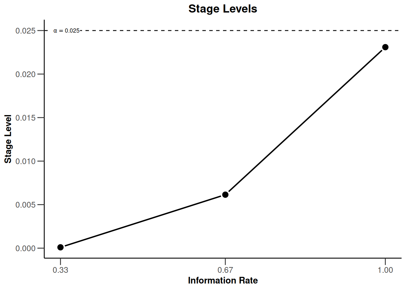
design |> plot(type = 4, showSource = TRUE)Source data of the plot (type 4):
x-axis: <environment>$informationRates
y-axis: <environment>$alphaSpent
Simple plot command example:
plot(<environment>$informationRates, <environment>$alphaSpent, type = "l")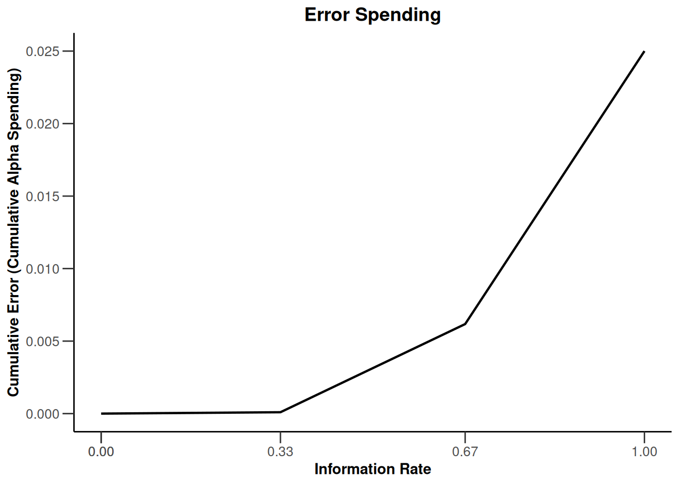
Decision regions for two-sided tests with futility bounds are displayed accordingly:
design <- getDesignGroupSequential(
    sided = 2,
    alpha = 0.05,
    beta = 0.2,
    informationRates = c(0.33, 0.67, 1),
    typeOfDesign = "asOF",
    typeBetaSpending = "bsP",
    bindingFutility = FALSE
)
design |> plot(type = 1)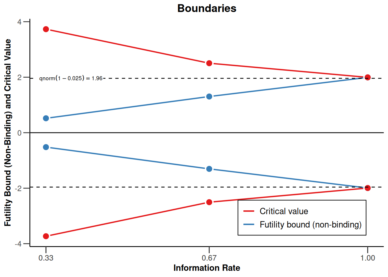
Comparison of multiple designs
Multiple designs can be combined into a design set (getDesignSet()) and their properties plotted jointly:
# O'Brien & Fleming, 3 equally spaced stages
d1 <- getDesignGroupSequential(
  typeOfDesign = "OF",
  kMax = 3
)
# Pocock
d2 <- getDesignGroupSequential(
  typeOfDesign = "P",
  kMax = 3
)
designSet <- getDesignSet(
  designs = c(d1, d2),
  variedParameters = "typeOfDesign"
)

designSet |> plot(type = 1)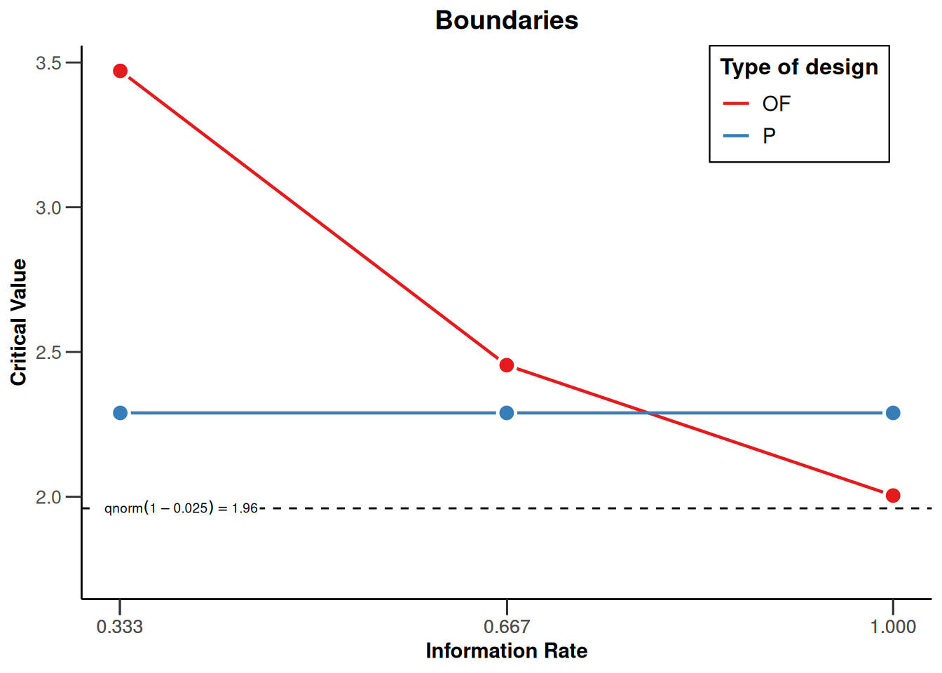
Even simpler, in rpact 3.0, you can also use plot(d1, d2).
System: rpact 4.4.0, R version 4.6.0 (2026-04-24), platform: x86_64-pc-linux-gnu
To cite R in publications use:
R Core Team (2026). R: A Language and Environment for Statistical Computing. R Foundation for Statistical Computing, Vienna, Austria. doi:10.32614/R.manuals https://doi.org/10.32614/R.manuals. https://www.R-project.org/.
To cite package ‘rpact’ in publications use:
Wassmer G, Pahlke F (2026). rpact: Confirmatory Adaptive Clinical Trial Design and Analysis. R package version 4.4.0. doi:10.32614/CRAN.package.rpact
Wassmer G, Brannath W (2025). Group Sequential and Confirmatory Adaptive Designs in Clinical Trials, 2nd edition. Springer, Cham, Switzerland. ISBN 978-3-031-89668-2. doi:10.1007/978-3-031-89669-9 https://doi.org/10.1007/978-3-031-89669-9.