library(rpact)
packageVersion("rpact") Simulation-Based Design of Group Sequential Trials with a Survival Endpoint with rpact
Planning
Survival
Power simulation
This document describes how to simulate design characterics for survival design under complex settings (incl. non-proportional hazards) in rpact.
Introduction
rpact provides the function getSimulationSurvival() for simulation of group sequential trials with a time-to-event endpoint. For a given scenario, getSimulationSurvival() simulates many hypothetical group sequential trials and calculates the test results. Based on this Monte Carlo simulation, estimates of key quantities such as overall study power, stopping probabilities at each interim analysis, timing of analyses etc. can be obtained.
getSimulationSurvival() complements the analytical calculations from the function getPowerSurvival() (and getSampleSizeSurvival()) in multiple ways:
- Simulations can be used to assess the accuracy of the analytical formulas.
- Simulations allow to answer questions such as the following:
- How variable is the timing of interim analysis (even if all assumptions are correct)?
- How could a dataset of a trial that is stopped early for efficacy at an interim analysis look like?
- Simulation is also possible for scenarios that are analytically intractable such as scenarios with delayed treatment effects.
The syntax of the function getSimulationSurvival() is very similar to the functions getPowerSurvival() and getSampleSizeSurvival(). Hence, this document only provides some examples and expects that the reader is familiar with the R Markdown document Designing group sequential trials with two groups and a survival endpoint with rpact which describes standard designs of a trial with a survival endpoint in rpact.
getSimulationSurvival() also supports the usage of adaptive sample size recalculation but this is not covered here. For more details, please also consult the help ?getSimulationSurvival.
First, load the rpact package
[1] '4.4.0'For this R Markdown document, some additional R packages are loaded which will be used to examine simulated datasets.
# Load ggplot2 for plotting
library(ggplot2) # general plotting
library(survminer) # plotting of KM curves with ggplot2
Loading required package: ggpubrlibrary(survival) # survival analysis routines
Attaching package: 'survival'The following object is masked from 'package:survminer':
myelomaStandard analytical calculation
For comparison with the simulation-based analysis, a standard example is first calculated under the following assumptions:
- Group-sequential design with one interim analysis after 66% of information using an O’Brien & Fleming type \(\alpha\)-spending function, one-sided Type I error 2.5%, power 80%:
design <- getDesignGroupSequential(
    informationRates = c(0.66, 1),
    typeOfDesign = "asOF",
    sided = 1,
    alpha = 0.025,
    beta = 0.2
)- Exponential PFS with a median PFS of 60 months in control (
median2 = 60) and a target hazard ratio of 0.74 (hazardRatio = 0.74). - Annual drop-out of 2.5% in both arms (
dropoutRate1 = 0.025, dropoutRate2 = 0.025, dropoutTime = 12). - Recruitment is 42 patients/month from month 6 onwards after linear ramp up. (
accrualTime = c(0,1,2,3,4,5,6), accrualIntensity = c(6,12,18,24,30,36,42)) - Randomization ratio 1:1 (
allocation1 = 1andallocation2 = 1); this is how subjects are randomized in treatment groups 1 and 2 in a subsequent way). 1:1 allocation is the default and is thus not explicitly set in the function call below. - A fixed total sample size of 1200 (
maxNumberOfSubjects = 1200).
As described in the vignette Designing group sequential trials with two groups and a survival endpoint with rpact, sample size calculations for this design can be performed as per the code below:
sampleSizeResult <- getSampleSizeSurvival(
  design,
  median2 = 60,
  hazardRatio = 0.74,
  dropoutRate1 = 0.025,
  dropoutRate2 = 0.025,
  dropoutTime = 12,
  accrualTime = c(0, 1, 2, 3, 4, 5, 6),
  accrualIntensity = c(6, 12, 18, 24, 30, 36, 42),
  maxNumberOfSubjects = 1200
)

# Summary of results
sampleSizeResult |> summary()
Sample size calculation for a survival endpoint
Sequential analysis with a maximum of 2 looks (group sequential design), one-sided overall significance level 2.5%, power 80%. The results were calculated for a two-sample logrank test, H0: hazard ratio = 1, H1: hazard ratio = 0.74, control median(2) = 60, maximum number of subjects = 1200, accrual time = c(1, 2, 3, 4, 5, 6, 31.571), accrual intensity = c(6, 12, 18, 24, 30, 36, 42), dropout rate(1) = 0.025, dropout rate(2) = 0.025, dropout time = 12.
| Stage | 1 | 2 |
|---|---|---|
| Planned information rate | 66% | 100% |
| Cumulative alpha spent | 0.0058 | 0.0250 |
| Stage levels (one-sided) | 0.0058 | 0.0232 |
| Efficacy boundary (z-value scale) | 2.524 | 1.992 |
| Efficacy boundary (t) | 0.718 | 0.808 |
| Cumulative power | 0.4074 | 0.8000 |
| Number of subjects | 1200.0 | 1200.0 |
| Expected number of subjects under H1 | 1200.0 | |
| Cumulative number of events | 231.3 | 350.5 |
| Expected number of events under H1 | 302.0 | |
| Analysis time | 39.54 | 53.65 |
| Expected study duration under H1 | 47.91 | |
| Exit probability for efficacy (under H0) | 0.0058 | |
| Exit probability for efficacy (under H1) | 0.4074 |
Legend:
- (t): treatment effect scale
By design, the power of the trial is 80%. The interim analysis is after 232 events which is expected to occur after 39.5 months, and the final analysis is after 351 events which is expected to occur after 53.7 months.
Use getPowerSurvival() to calculate the power achieved for the ceiled number of events. Note that the direction of the alternative needs to be specified. Here, the alternative is towards hazard ratios < 1 which is specified as directionUpper = FALSE.
powerResult <- getPowerSurvival(
  design,
  maxNumberOfEvents = ceiling(sampleSizeResult$maxNumberOfEvents),
  directionUpper = FALSE,
  median2 = 60,
  hazardRatio = 0.74,
  dropoutRate1 = 0.025,
  dropoutRate2 = 0.025,
  dropoutTime = 12,
  accrualTime = c(0, 1, 2, 3, 4, 5, 6),
  accrualIntensity = c(6, 12, 18, 24, 30, 36, 42),
  maxNumberOfSubjects = 1200
)

# Summary of results
powerResult |> summary()
Power calculation for a survival endpoint
Sequential analysis with a maximum of 2 looks (group sequential design), one-sided overall significance level 2.5%. The results were calculated for a two-sample logrank test, H0: hazard ratio = 1, power directed towards smaller values, H1: hazard ratio = 0.74, control median(2) = 60, maximum number of subjects = 1200, maximum number of events = 351, accrual time = c(1, 2, 3, 4, 5, 6, 31.571), accrual intensity = c(6, 12, 18, 24, 30, 36, 42), dropout rate(1) = 0.025, dropout rate(2) = 0.025, dropout time = 12.
| Stage | 1 | 2 |
|---|---|---|
| Planned information rate | 66% | 100% |
| Cumulative alpha spent | 0.0058 | 0.0250 |
| Stage levels (one-sided) | 0.0058 | 0.0232 |
| Efficacy boundary (z-value scale) | 2.524 | 1.992 |
| Efficacy boundary (t) | 0.718 | 0.808 |
| Cumulative power | 0.4080 | 0.8005 |
| Number of subjects | 1200.0 | 1200.0 |
| Expected number of subjects under H1 | 1200.0 | |
| Cumulative number of events | 231.7 | 351.0 |
| Expected number of events under H1 | 302.3 | |
| Analysis time | 39.58 | 53.72 |
| Expected study duration under H1 | 47.95 | |
| Exit probability for efficacy (under H0) | 0.0058 | |
| Exit probability for efficacy (under H1) | 0.4080 |
Legend:
- (t): treatment effect scale
These numbers will now be compared to simulations.
Simulation under proportional hazards
The call getSimulationSurvival() uses the same arguments as getSampleSizeSurvival() with the following changes:
- The maximum number of patients (
maxNumberOfSubjects = 1200) is always provided to allow the simulation. - The number of events at each analysis is specified as per the analytical calculation above (
plannedEvents = c(232,351)). - The direction of the alternative is specified as
directionUpper = FALSE. - The number of simulated trials is specified (
maxNumberOfIterations = 10000in the example below). - By default, raw datasets from simulation runs are not extracted. However, in this example, it is specified that one raw dataset that led to stopping after each stage, respectively, will be stored:
maxNumberOfRawDatasetsPerStage = 1. - For reproducibility, it is useful to set the random seed which is set to
seed = 234in the example. - For simulation of trials with unequal randomization, integer arguments
allocation1andallocation2must be provided to the functiongetSimulationSurvival(instead of argumentallocationRatioPlannedin the functiongetSampleSizeSurvival).allocation1andallocation2specify the number of consecutively enrolled subjects in the intervention and control groups, respectively, before another subject from the opposite group is recruited. For example,allocation1 = 2, allocation2 = 1refers to 2 (intervention):1 (control) randomization andallocation1 = 1, allocation2 = 2to 1 (intervention):2 (control) randomization.
simulationResult <- getSimulationSurvival(
    design,
    median2 = 60,
    hazardRatio = 0.74,
    dropoutRate1 = 0.025,
    dropoutRate2 = 0.025,
    dropoutTime = 12,
    accrualTime = c(0, 1, 2, 3, 4, 5, 6),
    accrualIntensity = c(6, 12, 18, 24, 30, 36, 42),
    plannedEvents = c(232, 351),
    directionUpper = FALSE,
    maxNumberOfSubjects = 1200,
    maxNumberOfIterations = 10000,
    maxNumberOfRawDatasetsPerStage = 1,
    seed = 234
)

# Summary of simulation results
simulationResult |> summary()
Simulation of a survival endpoint
Sequential analysis with a maximum of 2 looks (group sequential design), one-sided overall significance level 2.5%. The results were simulated for a two-sample logrank test, H0: hazard ratio = 1, power directed towards smaller values, H1: hazard ratio = 0.74, control median(2) = 60, planned cumulative events = c(232, 351), maximum number of subjects = 1200, accrual time = c(1, 2, 3, 4, 5, 6, 31.571), accrual intensity = c(6, 12, 18, 24, 30, 36, 42), dropout rate(1) = 0.025, dropout rate(2) = 0.025, dropout time = 12, simulation runs = 10000, seed = 234.
| Stage | 1 | 2 |
|---|---|---|
| Planned information rate | 66% | 100% |
| Cumulative alpha spent | 0.0058 | 0.0250 |
| Stage levels (one-sided) | 0.0058 | 0.0232 |
| Efficacy boundary (z-value scale) | 2.524 | 1.992 |
| Cumulative power | 0.3974 | 0.7959 |
| Number of subjects | 1200.0 | 1200.0 |
| Expected number of subjects under H1 | 1200.0 | |
| Cumulative number of events | 232.0 | 351.0 |
| Expected number of events under H1 | 303.7 | |
| Analysis time | 39.61 | 53.66 |
| Expected study duration under H1 | 48.09 | |
| Conditional power (achieved) | 0.5446 | |
| Exit probability for efficacy | 0.3974 |
According to the output, the simulated overall power is 79.6% and the probability to cross the efficacy boundary at the interim analysis is 39.7%. These are both within 1% of the analytical power.
The mean simulated analysis times are after 39.61 months for the interim analysis and after 53.66 for the final analysis. Both timings differ by <0.1 months from the analytical calculation (Difference analysis times = 0.06, 0.01).
You can show median [range] and mean+/-sd of the trial results across the simulated datasets with the print() command together showStatistics = TRUE:
# Print of simulation results showing trial results statistics
simulationResult |> print(showStatistics = TRUE)
Simulation of survival data (group sequential design)
Design parameters
- Information rates: 0.660, 1.000
- Critical values: 2.524, 1.992
- Futility bounds (non-binding): -Inf
- Cumulative alpha spending: 0.005798, 0.025000
- Local one-sided significance levels: 0.005798, 0.023210
- Significance level: 0.0250
- Test: one-sided
User defined parameters
- Maximum number of iterations: 10000
- Seed: 234
- Direction upper: FALSE
- Planned cumulative events: 232, 351
- Accrual intensity: 6.0, 12.0, 18.0, 24.0, 30.0, 36.0, 42.0
- Drop-out rate (1): 0.025
- Drop-out rate (2): 0.025
- Hazard ratio: 0.740
- Maximum number of subjects: 1200
- median(2): 60.0
Default parameters
- Planned allocation ratio: 1
- Conditional power: NA
- Allocation 1: 1
- Allocation 2: 1
- Drop-out time: 12.00
- kappa: 1
- Theta H0: 1
Results
- Accrual time: 1.00, 2.00, 3.00, 4.00, 5.00, 6.00, 31.57
- Analysis time [1]: 39.61
- Analysis time [2]: 53.66
- Events not achieved [1]: 0.000
- Events not achieved [2]: 0.000
- lambda(1): 0.00855
- lambda(2): 0.0116
- median(1): 81.1
- Assumed treatment rate: 0.0975
- Assumed control rate: 0.129
- Expected study duration: 48.09
- Cumulative number of events [1]: 232
- Cumulative number of events [2]: 351
- Iterations [1]: 10000
- Iterations [2]: 6026
- Overall reject: 0.7959
- Reject per stage [1]: 0.3974
- Reject per stage [2]: 0.3985
- Overall futility stop: 0.0000
- Futility stop per stage: 0.0000
- Early stop: 0.3974
- Expected number of subjects: 1200
- Expected number of events: 303.7
- Number of subjects [1]: 1200
- Number of subjects [2]: 1200
- Conditional power (achieved) [1]: NA
- Conditional power (achieved) [2]: 0.5446
Simulated data
- Analysis time [1] : median [range]: 39.578 [33.988 - 45.552]; mean +/-sd: 39.606 +/-1.47; n = 10000
- Analysis time [2] : median [range]: 53.616 [46.872 - 61.013]; mean +/-sd: 53.659 +/-2.007; n = 6026
- Number of subjects [1] : median [range]: 1200 [1200 - 1200]; mean +/-sd: 1200 +/-0; n = 10000
- Number of subjects [2] : median [range]: 1200 [1200 - 1200]; mean +/-sd: 1200 +/-0; n = 6026
- Test statistic [1] : median [range]: 2.267 [-1.52 - 5.611]; mean +/-sd: 2.269 +/-0.99; n = 10000
- Test statistic [2] : median [range]: 2.314 [-0.877 - 4.832]; mean +/-sd: 2.282 +/-0.773; n = 6026
- Log-rank statistic [1] : median [range]: 2.267 [-1.52 - 5.611]; mean +/-sd: 2.269 +/-0.99; n = 10000
- Log-rank statistic [2] : median [range]: 2.314 [-0.877 - 4.832]; mean +/-sd: 2.282 +/-0.773; n = 6026
- Hazard ratio estimate LR [1] : median [range]: 0.743 [0.479 - 1.221]; mean +/-sd: 0.749 +/-0.098; n = 10000
- Hazard ratio estimate LR [2] : median [range]: 0.781 [0.597 - 1.098]; mean +/-sd: 0.787 +/-0.066; n = 6026
- Conditional power (achieved) [2] : median [range]: 0.607 [0 - 0.972]; mean +/-sd: 0.545 +/-0.336; n = 6026
Legend
- (i): values of treatment arm i
- [k]: values at stage k
Accessing trial summaries per stage for each simulation
Summary results for each trial can be obtained from the simulation object using the function getData(). Similarly, raw data from individual trials that were stopped at each stage can be obtained using the function getRawData() (if maxNumberOfRawDatasetsPerStage was set > 0). The format of these datasets is described in the help ?getSimulationSurvival and illustrated now.
# get aggregate datasets from all simulation runs
aggregateSimulationData <- getData(simulationResult)
# show the first 6 records of the dataset
head(aggregateSimulationData)| iterationNumber | 1 | 1 | 2 | 3 | 3 | 4 |
| stageNumber | 1 | 2 | 1 | 1 | 2 | 1 |
| pi1 | 0.1 | 0.1 | 0.1 | 0.1 | 0.1 | 0.1 |
| pi2 | 0.1 | 0.1 | 0.1 | 0.1 | 0.1 | 0.1 |
| hazardRatio | 0.74 | 0.74 | 0.74 | 0.74 | 0.74 | 0.74 |
| analysisTime | 40.07 | 53.85 | 41.22 | 40.62 | 54.54 | 40.74 |
| numberOfSubjects | 1200 | 1200 | 1200 | 1200 | 1200 | 1200 |
| overallEvents1 | 100 | 159 | 94 | 107 | 165 | 98 |
| overallEvents2 | 132 | 192 | 138 | 125 | 186 | 134 |
| eventsPerStage | 232 | 119 | 232 | 232 | 119 | 232 |
| rejectPerStage | 0 | 1 | 1 | 0 | 0 | 1 |
| eventsNotAchieved | 0 | 0 | 0 | 0 | 0 | 0 |
| futilityPerStage | 0 | 0 | 0 | 0 | 0 | 0 |
| testStatistic | 2.474 | 2.328 | 3.162 | 1.446 | 1.558 | 2.724 |
| logRankStatistic | 2.474 | 2.328 | 3.162 | 1.446 | 1.558 | 2.724 |
| conditionalPowerAchieved | NA | 0.9644 | NA | NA | 0.3572 | NA |
| pValuesSeparate | NA | NA | NA | NA | NA | NA |
| trialStop | FALSE | TRUE | TRUE | FALSE | TRUE | TRUE |
| hazardRatioEstimateLR | 0.7226 | 0.7800 | 0.6602 | 0.8271 | 0.8468 | 0.6993 |
# The aggregated dataset contains one record for each of the 10'000 simulated
# interim datasets (stageNumber = 1), and one additional record for the final
# analysis (stageNumber = 2) for all simulated trials which were not stopped at
# the interim analysis
table(aggregateSimulationData$stageNumber)
    1     2
10000  6026
# One possible analysis which uses the aggregated dataset:
# display the distribution of the timing of the analyses (by stage)
# across simulation runs
p <- ggplot(aggregateSimulationData, aes(factor(stageNumber), analysisTime))
p + geom_boxplot() + labs(
x = "Analysis stage",
y = "Timing of analysis (months \nfrom first patient randomized)"
)
Accessing summaries for a simulated trial stopped at interim
# Get all stored raw datasets
rawSimulationDataData <- getRawData(simulationResult)

# Choose one dataset which corresponds to a simulated (hypothetical) trial
# which was stopped at the efficacy interim analysis
# (only 1 such dataset exists here, because maxNumberOfRawDatasetsPerStage
# was set to 1 above)
stage1rawData <- subset(rawSimulationDataData, stopStage == 1)

# Perform a Cox regression analysis of the simulated trial
# (treatmentGroup == 1 is the intervention arm)
# Note that the $p$-value from the Cox regression is two-sided whereas
# the group sequential test is one-sided.
summary(coxph(Surv(timeUnderObservation, event) ~ I(treatmentGroup == 1),
    data = stage1rawData
))
Call:
coxph(formula = Surv(timeUnderObservation, event) ~ I(treatmentGroup ==
1), data = stage1rawData)
n= 1200, number of events= 232
coef exp(coef) se(coef) z Pr(>|z|)
I(treatmentGroup == 1)TRUE -0.4199 0.6571 0.1337 -3.139 0.00169 **
---
Signif. codes: 0 '***' 0.001 '**' 0.01 '*' 0.05 '.' 0.1 ' ' 1
exp(coef) exp(-coef) lower .95 upper .95
I(treatmentGroup == 1)TRUE 0.6571 1.522 0.5056 0.8541
Concordance= 0.553 (se = 0.017 )
Likelihood ratio test= 10.05 on 1 df, p=0.002
Wald test = 9.85 on 1 df, p=0.002
Score (logrank) test = 10 on 1 df, p=0.002# Show Kaplan-Meier curves of the simulated trial
ggsurvplot(
survfit(Surv(timeUnderObservation, event) ~ treatmentGroup,
data = stage1rawData
),
pval = TRUE,
risk.table = TRUE,
break.time.by = 12,
censor.size = 1,
risk.table.y.text.col = TRUE,
risk.table.fontsize = 3,
legend.labs = c("Treatment", "Control"),
title = paste0(
"Kaplan-Meier curve of one simulated trial\n which ",
"was stopped at the interim analysis"
),
xlab = "Time (months)", data = stage1rawData
)Ignoring unknown labels:
• colour : "Strata"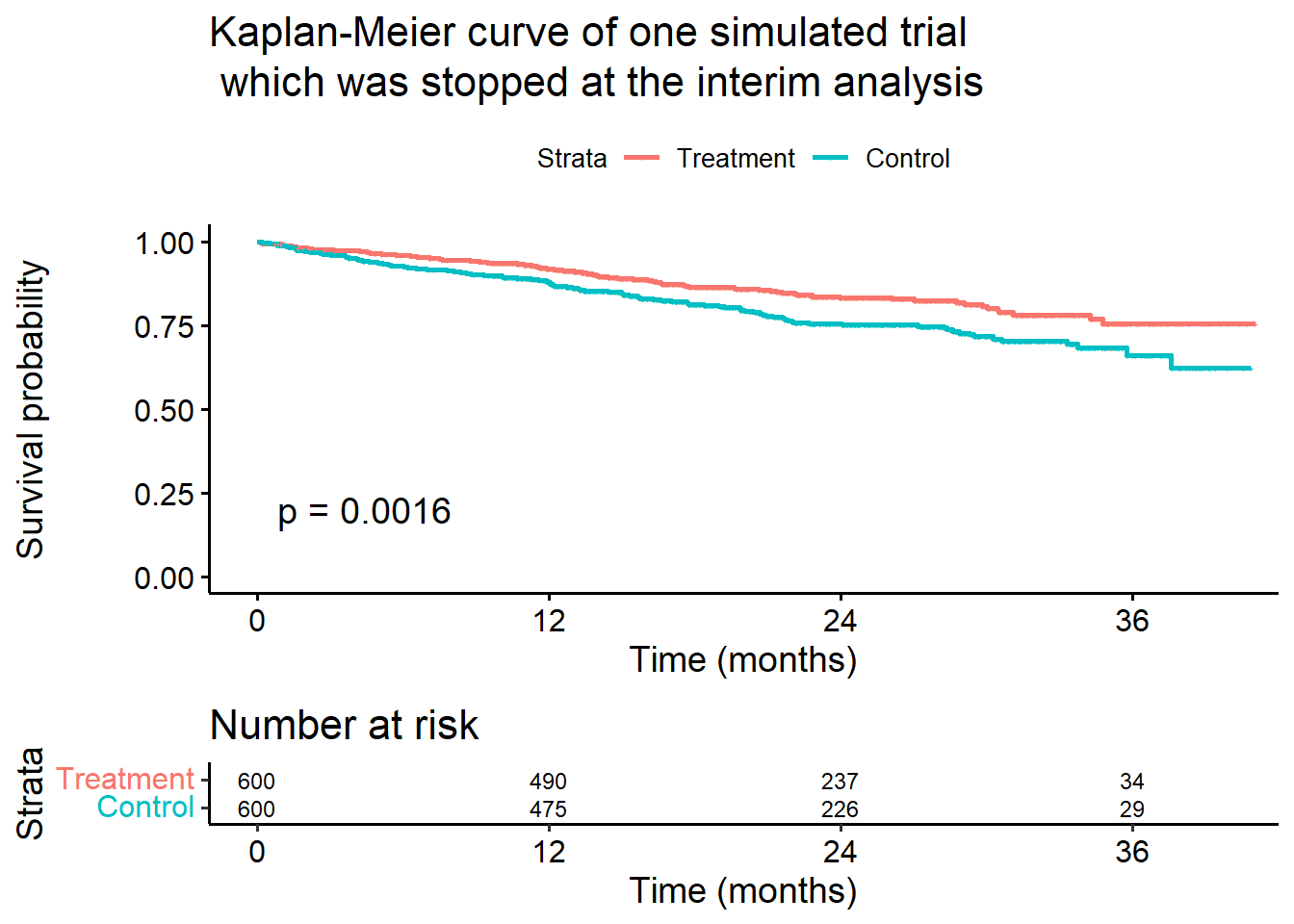
Simulation under non-proportional hazards
For the sake of illustration, assume that the treatment effect in the example above is delayed by 6 months, i.e., that the active treatment does not affect the hazard in the first 6 months but still reduces it by 0.74-fold from month 6 onwards. The code below determines the power of the design in this situation via simulation.
The code to specify a delayed treatment effect is similar to the simulation under proportional hazards except that now the survival function in each arm is specified via a piecewise constant exponential distribution defined through the hazard rates (not the medians):
piecewiseSurvivalTime = c(0,6),
lambda2 = c(log(2)/60,log(2)/60),
lambda1 = c(log(2)/60,0.74*log(2)/60)
(as always for rpact, “2” refers to the control arm which still has a constant hazard rate, i.e., an exponential distribution).
# Simulation assuming a delayed treatment effect
simulationResultNPH <- getSimulationSurvival(
  design,
  piecewiseSurvivalTime = c(0, 6),
  lambda2 = c(log(2) / 60, log(2) / 60),
  lambda1 = c(log(2) / 60, 0.74 * log(2) / 60),
  dropoutRate1 = 0.025,
  dropoutRate2 = 0.025,
  dropoutTime = 12,
  accrualTime = c(0, 1, 2, 3, 4, 5, 6),
  accrualIntensity = c(6, 12, 18, 24, 30, 36, 42),
  plannedEvents = c(232, 351),
  directionUpper = FALSE,
  maxNumberOfSubjects = 1200,
  maxNumberOfIterations = 10000,
  maxNumberOfRawDatasetsPerStage = 1,
  seed = 234
)
simulationResultNPH |> summary()
Simulation of a survival endpoint
Sequential analysis with a maximum of 2 looks (group sequential design), one-sided overall significance level 2.5%. The results were simulated for a two-sample logrank test, H0: hazard ratio = 1, power directed towards smaller values, H1: hazard ratio = c(1, 0.74), piecewise survival distribution, piecewise survival time = c(0, 6), control lambda(2) = c(0.0116, 0.0116), planned cumulative events = c(232, 351), maximum number of subjects = 1200, accrual time = c(1, 2, 3, 4, 5, 6, 31.571), accrual intensity = c(6, 12, 18, 24, 30, 36, 42), dropout rate(1) = 0.025, dropout rate(2) = 0.025, dropout time = 12, simulation runs = 10000, seed = 234.
| Stage | 1 | 2 |
|---|---|---|
| Planned information rate | 66% | 100% |
| Cumulative alpha spent | 0.0058 | 0.0250 |
| Stage levels (one-sided) | 0.0058 | 0.0232 |
| Efficacy boundary (z-value scale) | 2.524 | 1.992 |
| Cumulative power | 0.1525 | 0.5671 |
| Number of subjects | 1200.0 | 1200.0 |
| Expected number of subjects under H1 | 1200.0 | |
| Cumulative number of events | 232.0 | 351.0 |
| Expected number of events under H1 | 332.9 | |
| Analysis time | 38.64 | 52.63 |
| Expected study duration under H1 | 50.53 | |
| Conditional power (achieved) | 0.3512 | |
| Exit probability for efficacy | 0.1525 |
As can be seen from the output above, power drops substantially to 56.7%.
If one wants the trial to maintain a power of 80% despite the delayed treatment effect, the maximal number of events would need to be increased and some experimentation shows that one would need 498 events in this case as demonstrated in the simulation below. Note further that in this non-proportional hazards scenario, power does not only depend on the number of events but also on other assumptions, in particular on assumptions regarding the speed of recruitment.
# Simulation assuming a delayed treatment effect
plannedEventsMax <- 498
simulationResultNPH2 <- getSimulationSurvival(
  design,
  piecewiseSurvivalTime = c(0, 6),
  lambda2 = c(log(2) / 60, log(2) / 60),
  lambda1 = c(log(2) / 60, 0.74 * log(2) / 60),
  dropoutRate1 = 0.025,
  dropoutRate2 = 0.025,
  dropoutTime = 12,
  accrualTime = c(0, 1, 2, 3, 4, 5, 6),
  accrualIntensity = c(6, 12, 18, 24, 30, 36, 42),
  plannedEvents = c(ceiling(0.66 * plannedEventsMax), plannedEventsMax),
  directionUpper = FALSE,
  maxNumberOfSubjects = 1200,
  maxNumberOfIterations = 10000,
  maxNumberOfRawDatasetsPerStage = 1,
  seed = 456
)
simulationResultNPH2 |> summary()
Simulation of a survival endpoint
Sequential analysis with a maximum of 2 looks (group sequential design), one-sided overall significance level 2.5%. The results were simulated for a two-sample logrank test, H0: hazard ratio = 1, power directed towards smaller values, H1: hazard ratio = c(1, 0.74), piecewise survival distribution, piecewise survival time = c(0, 6), control lambda(2) = c(0.0116, 0.0116), planned cumulative events = c(329, 498), maximum number of subjects = 1200, accrual time = c(1, 2, 3, 4, 5, 6, 31.571), accrual intensity = c(6, 12, 18, 24, 30, 36, 42), dropout rate(1) = 0.025, dropout rate(2) = 0.025, dropout time = 12, simulation runs = 10000, seed = 456.
| Stage | 1 | 2 |
|---|---|---|
| Planned information rate | 66% | 100% |
| Cumulative alpha spent | 0.0058 | 0.0250 |
| Stage levels (one-sided) | 0.0058 | 0.0232 |
| Efficacy boundary (z-value scale) | 2.524 | 1.992 |
| Cumulative power | 0.3269 | 0.7958 |
| Number of subjects | 1200.0 | 1200.0 |
| Expected number of subjects under H1 | 1200.0 | |
| Cumulative number of events | 329.0 | 498.0 |
| Expected number of events under H1 | 442.8 | |
| Analysis time | 49.87 | 74.11 |
| Expected study duration under H1 | 66.22 | |
| Conditional power (achieved) | 0.4867 | |
| Exit probability for efficacy | 0.3269 |
System: rpact 4.4.0, R version 4.5.3 (2026-03-11), platform: x86_64-pc-linux-gnu
To cite R in publications use:
R Core Team (2026). R: A Language and Environment for Statistical Computing. R Foundation for Statistical Computing, Vienna, Austria. https://www.R-project.org/.
To cite package ‘rpact’ in publications use:
Wassmer G, Pahlke F (2026). rpact: Confirmatory Adaptive Clinical Trial Design and Analysis. R package version 4.4.0. doi:10.32614/CRAN.package.rpact
Wassmer G, Brannath W (2025). Group Sequential and Confirmatory Adaptive Designs in Clinical Trials, 2nd edition. Springer, Cham, Switzerland. ISBN 978-3-031-89668-2, doi:10.1007/978-3-031-89669-9 https://doi.org/10.1007/978-3-031-89669-9.